Pricing a Single Product

September 20, 2026

One number to set. Raise the price and you make more on each sale, but fewer people buy — so profit traces an inverted U. This post finds the top of that curve and gives you a benchmark you can estimate without a calculator.

Price Optimization · Part 1 of 4 · 12 min read

← First part　·　Series index　·　Pricing Many Items Under Constraints →

This is the first post in A Primer on Price Optimization. No background is needed — just the fact that the more something costs, the fewer people buy it.

Symbols used in this post

Symbol	Meaning
$p$	Price, the decision variable
$c$	Unit cost, a known constant
$q(p)$	Purchase probability / conversion rate, decreasing in $p$
$k$	Price coefficient: the larger it is, the faster conversion drops when the price moves
$\Pi$	Total profit (gross margin throughout this series, not revenue)
$q_0 = 1-q$	Probability of no purchase

The full notation table is in the series index.

1. Setting up the problem

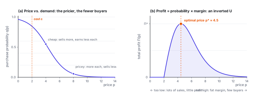
There's a single pricing unit, with its own price–demand curve: the higher the price, the lower the chance of a sale.

q = q(p), \qquad q'(p) < 0

With a fixed unit cost $c$ , total profit is

\boxed{\ \Pi(p) = \underbrace{q(p)}_{\text{purchase probability}} \times \underbrace{(p - c)}_{\text{margin per order}}\ }

There's a built-in tension in this formula:

Raise the price → you make more on each order ( $p-c$ grows)
Raise the price → fewer people buy ( $q$ shrinks)

Multiply the two and you usually get an inverted U: too cheap and you don't make money, too expensive and nobody buys, with a peak somewhere in between.

The price–demand curve and total profit

2. Finding the optimum

Differentiate with respect to $p$ and set the derivative to zero:

\frac{d\Pi}{dp} = \underbrace{q(p)}_{\text{①}} + \underbrace{(p-c)\,q'(p)}_{\text{②}} = 0

Each term has a clear meaning:

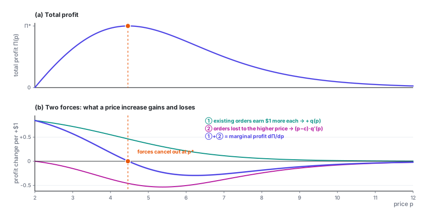
① $q(p)$ : each extra dollar of price earns one more dollar on the orders you were already getting — $q$ in total. This is the gain, and it's always positive.
② $(p-c)q'(p)$ : each extra dollar of price loses $|q'(p)|$ orders, each of which was worth a margin of $(p-c)$ . This is the loss, and it's negative whenever the price is above cost.

The optimal price is the point where these two forces exactly cancel out.

The two forces behind a price increase

Rearranging gives the general condition the optimal price has to satisfy:

\boxed{\ p^\star = c + \frac{q(p^\star)}{-\,q'(p^\star)}\ }

In words: optimal price = cost + a markup, where

\text{markup} \;=\; \frac{\text{current conversion rate}}{\text{rate at which conversion falls}}

This matches intuition: the more slowly conversion falls (the less customers care about price), the more room you have to mark up.

The same formula shows up twice in ad auctions. A platform setting a reserve price faces exactly this problem, with a cost of zero; and a buyer's optimal first-price bid, $b^\star = v - w/w'$ , is its mirror image, shading down from value instead of marking up from cost. See Part 1 of the ad bidding series.

3. Two worked examples

That was the general form. Plug in a specific demand function and you get a formula you can actually compute.

Example 1: linear demand

q(p) = a - b\,p \qquad (a, b > 0)

Substitute into the objective:

\Pi(p) = (a - bp)(p - c) = -bp^2 + (a + bc)\,p - ac

This is a downward-opening parabola. Differentiate:

\frac{d\Pi}{dp} = -2bp + (a + bc) = 0

\boxed{\ p^\star = \frac{a + bc}{2b} = \frac{a}{2b} + \frac{c}{2}\ }

The second derivative is $\frac{d^2\Pi}{dp^2} = -2b < 0$ , so this is indeed a maximum.

There's a neat way to put this. Let $p_{\max} = a/b$ be the "zero-demand price" (at this price, nobody buys at all). Then

p^\star = \frac{p_{\max} + c}{2}

The optimal price is exactly halfway between your cost and the zero-demand price. That makes a very handy mental benchmark: if you can estimate the price at which nothing sells anymore, the optimal price is roughly midway between that and your cost.

Example 2: logit demand (closer to reality)

Linear demand has a flaw: push the price a little higher and $q$ goes negative. In practice, the logit form is more common:

q(p) = \frac{1}{1 + e^{-(b_0 - k p)}} = \sigma(b_0 - kp)

Here $\sigma(\cdot)$ is the sigmoid function, $b_0$ sets the baseline appeal, and $k > 0$ is the price coefficient. It naturally stays within $(0,1)$ and decreases with price.

It has a very convenient derivative:

q'(p) = \frac{dq}{dp} = -k\,q\,(1-q)

Show: where this comes from

Let $z = b_0 - kp$ , so that $q = \sigma(z) = \frac{1}{1+e^{-z}}$ .

The sigmoid has the classic property $\sigma'(z) = \sigma(z)\bigl(1-\sigma(z)\bigr)$ :

\sigma'(z) = \frac{e^{-z}}{(1+e^{-z})^2} = \frac{1}{1+e^{-z}} \cdot \frac{e^{-z}}{1+e^{-z}} = \sigma(z)\bigl(1-\sigma(z)\bigr)

Then apply the chain rule, with $\frac{dz}{dp} = -k$ :

\frac{dq}{dp} = \sigma'(z)\cdot\frac{dz}{dp} = q(1-q)\cdot(-k) = -k\,q(1-q)

Plug this into the first-order condition $q + (p-c)q' = 0$ :

q - (p-c)\,k\,q\,(1-q) = 0

Divide both sides by $q$ (fine, since $q > 0$ ):

1 - k\,(p-c)(1-q) = 0

\boxed{\ p^\star - c = \frac{1}{k\,\bigl(1 - q(p^\star)\bigr)} = \frac{1}{k\,q_0}\ }

where $q_0 = 1 - q$ is the probability of no purchase.

This is an implicit equation (the right-hand side still depends on $p^\star$ ), but it has a single unknown and is monotone, so bisection or Newton's method converges in a few steps. In practice, it's a non-issue.

4. Reading the formulas in business terms

Reading 1: the larger $k$ , the smaller the markup.

$k$ is the price coefficient. A large $k$ means price-sensitive customers, a steep curve, and a big drop in volume from even a small price increase — so the formula tells you to keep the markup modest. Conversely, when customers don't much care about price (must-haves, no alternatives, urgent needs), $1/k$ is large and so is the room to mark up.

Reading 2: $q_0$ sits in the denominator, so how well you're selling right now feeds back into what you should charge.

This one is easy to misread, so it's worth spelling out. Suppose almost everyone buys at your current price ( $q \to 1$ , $q_0 \to 0$ ). The formula then calls for an almost infinite markup. It isn't broken — it's telling you that your price is too low. Once you raise the price, $q$ falls, $q_0$ rises, and the markup the formula asks for shrinks; the optimum is where the two meet. So don't treat it as a one-shot formula: the right-hand side depends on $p^\star$ , and you solve it with bisection or Newton's method, as in the previous section.

Reading 3: the answer is sensitive to how you count cost.

What goes into $c$ ? Only variable costs, or allocated fixed costs too? That choice moves the optimal price directly. As a rule, for short-term pricing decisions $c$ should include only marginal cost — the extra cost of making one more sale. Folding fixed costs in before optimizing systematically pushes prices too high and volume too low.

5. Pitfalls in practice

The curve doesn't fall from the sky. Every derivation above assumes you know $q(p)$ . That's much harder than it looks; Part 4 goes into it.
$c$ may not be constant. In many businesses cost changes with volume (economies of scale, tiered capacity, inventory tiers). Then $\Pi = q\cdot(p - c(q))$ , and you need to redo the derivative, but the framework stays the same.
Don't forget the second-order condition. A zero first derivative only gives you a stationary point. Under logit demand, $\Pi(p)$ is not necessarily concave in $p$ everywhere, but it is unimodal, so the solution of the first-order condition is the global optimum.

Show: a trick that makes every later algorithm simpler — change the variable and the problem becomes concave

$\Pi(p)$ isn't necessarily concave in $p$ , which makes optimization algorithms awkward to write. But if you switch the decision variable from price to conversion rate, the problem becomes strictly concave right away.

Invert $q = \sigma(b_0 - kp)$ to get the price:

p = \frac{1}{k}\left(b_0 - \ln\frac{q}{1-q}\right)

Substitute back into the objective:

\Pi(q) = q\left(\frac{b_0}{k} - c\right) - \frac{1}{k}\underbrace{\left(q\ln q - q\ln(1-q)\right)}_{\;\equiv\, f(q)}

The first term is linear in $q$ , so if $f(q)$ is convex, $\Pi(q)$ is concave:

f'(q) = \ln q + 1 - \ln(1-q) + \frac{q}{1-q}

f''(q) = \frac{1}{q} + \frac{1}{1-q} + \frac{1}{(1-q)^2} \;>\; 0 \quad \text{(for all } 0<q<1 \text{)}

So $\Pi''(q) = -f''(q)/k < 0$ : strictly concave.

Why this matters in practice: once the problem is concave in $q$ , you can hand it straight to a convex optimization solver, with a guaranteed global optimum and no worries about starting points or local optima. It's also, at heart, why the Lagrangian derivation in Part 3 comes out so clean.

Price Optimization · Part 1 of 4

← First part　·　Series index　·　Pricing Many Items Under Constraints →

Revision history