Pricing Substitutable Products

September 20, 2026

Raise the price of one product and another one sells more — they're competing for the same demand. Once prices are linked like this, you can no longer set them one at a time. Yet the optimum turns out to be surprisingly clean: every product's marginal unit economics, what one more sale of it nets you, has to sit at the same water level.

Price Optimization · Part 3 of 4 · 13 min read

← Pricing Many Items Under Constraints　·　Series index　·　Pricing at Scale →

Previously: the first two posts assumed that changing one unit's price doesn't affect any other unit. This post drops that assumption — when users face a whole list of options, those options take volume from each other.

Symbols used in this post

Symbol	Meaning
$u_j = p_j - c_j$	Margin per order of option $j$
$b_j$	Appeal that has nothing to do with price (brand, word of mouth, ratings…)
$D$	Logit denominator, $D = 1 + \sum_m e^{\,b_m - k_m p_m}$
$q_j = e^{\,b_j-k_jp_j}/D$	Probability of choosing option $j$
$q_0 = 1/D$	Probability of buying nothing
$\mathrm{mUE}_j$	Marginal unit economics: how much more you net if $j$ sells one more unit, $u_j - 1/k_j$ (the adjusted markup in the literature)

The full notation table is in the series index.

1. What changes

Everything in the first two posts rests on one assumption: changing one unit's price doesn't change any other unit's conversion rate.

Real life often isn't like that. A user rarely faces a single option; they face a whole list of candidates (a screen of products, a set of plans, a lineup of car models, a menu of insurance policies). And then:

Raise the price of the first item on the list, and the user doesn't necessarily walk away — they may simply buy the second item instead.

So change one price, and the conversion rate of every item on the list moves.

This effect goes by different names in different fields:

In economics, it's the cross-price effect, and the options are substitutes
In retail and revenue management, it's cannibalization: your own products taking volume from each other
Mathematically, the off-diagonal entries of the Hessian (or the demand Jacobian) are no longer zero

Of the three decoupling conditions from the beginning of Part 2, this is the third one breaking.

2. Modeling it with a discrete choice model

The standard tool is the multinomial logit model (MNL).

The user faces $N$ options plus a "buy nothing" option. The probability of choosing option $j$ is:

\boxed{\ q_j \;=\; \frac{e^{\,b_j - k_j p_j}}{\underbrace{1}_{\text{buy nothing}} + \sum_{m=1}^{N} e^{\,b_m - k_m p_m}}\ }

Numerator: option $j$ 's own appeal, which shrinks as its price rises
The lone 1 in the denominator: the outside option (not buying). It anchors the whole model. Without it, a price increase could only push users from one option to another, total volume would never fall, and the model would be unrealistic
$b_j$ : appeal that has nothing to do with price (brand, word of mouth, ratings, delivery speed…)
$k_j$ : option $j$ 's price coefficient

To keep the notation short, write:

D = 1 + \sum_m e^{\,b_m - k_m p_m}, \qquad e_j = e^{\,b_j - k_j p_j}, \qquad q_j = \frac{e_j}{D}, \qquad q_0 = \frac{1}{D}

$q_0$ is the probability of buying nothing, and clearly $q_0 + \sum_j q_j = 1$ .

3. The derivatives: what substitution looks like

Everything later builds on these, so let's go step by step.

Own-price derivative (how changing $p_j$ affects $q_j$ itself):

\frac{\partial q_j}{\partial p_j} = \frac{\partial}{\partial p_j}\left(\frac{e_j}{D}\right) = \frac{\frac{\partial e_j}{\partial p_j}\cdot D - e_j\cdot\frac{\partial D}{\partial p_j}}{D^2}

Here $\frac{\partial e_j}{\partial p_j} = -k_j e_j$ , and $\frac{\partial D}{\partial p_j} = -k_j e_j$ (only the $j$ -th term of $D$ contains $p_j$ ). Substituting:

= \frac{-k_je_jD + k_je_j^2}{D^2} = -k_j\frac{e_j}{D}\left(1 - \frac{e_j}{D}\right)

\boxed{\ \frac{\partial q_j}{\partial p_j} = -k_j\,q_j\,(1 - q_j) \;<\; 0\ }

Cross-price derivative (how changing $p_j$ affects another option's $q_m$ , with $m \ne j$ ):

The numerator $e_m$ doesn't depend on $p_j$ ; only the denominator moves:

\frac{\partial q_m}{\partial p_j} = e_m\cdot\frac{\partial}{\partial p_j}\left(\frac{1}{D}\right) = -\frac{e_m}{D^2}\cdot\frac{\partial D}{\partial p_j} = -\frac{e_m}{D^2}\cdot(-k_je_j)

\boxed{\ \frac{\partial q_m}{\partial p_j} = k_j\,q_j\,q_m \;>\; 0\ }

These two formulas are substitution written in math: raise your own price and you lose volume (negative); everyone else gains (positive).

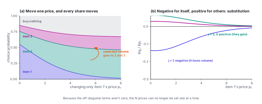
Substitution: move one price and every share moves

One more quantity we'll need later — the effect of raising $p_j$ on total volume:

\sum_{m}\frac{\partial q_m}{\partial p_j} = \underbrace{-k_jq_j(1-q_j)}_{m=j} + \underbrace{\sum_{m\ne j}k_jq_jq_m}_{m \ne j} = -k_jq_j\Bigl(1 - \sum_m q_m\Bigr)

\boxed{\ \sum_m \frac{\partial q_m}{\partial p_j} = -\,k_j\,q_j\,q_0\ }

A lovely result: of the volume that walks away after a price increase, only the part that leaks into "buy nothing" is really lost; moves between options don't count as losses.

4. Finding the optimum: the knob in explicit form

The objective (with margin per order $u_j = p_j - c_j$ ):

\Pi = \sum_j q_j\,u_j

Differentiate with respect to $p_j$ . Note that $p_j$ acts through two channels: directly, on its own margin $u_j$ ; and through the shares, on every $q_m$ :

\frac{\partial \Pi}{\partial p_j} = \underbrace{q_j}_{\text{margin effect}} + \underbrace{\sum_m u_m\frac{\partial q_m}{\partial p_j}}_{\text{share effect}}

Plug in the derivatives:

= q_j + u_j\bigl(-k_jq_j(1-q_j)\bigr) + \sum_{m\ne j}u_m\,k_jq_jq_m

Factor out $q_j$ :

= q_j\left[1 - k_ju_j(1-q_j) + k_j\sum_{m\ne j}u_mq_m\right]

Expand $(1-q_j)$ :

= q_j\left[1 - k_ju_j + k_ju_jq_j + k_j\sum_{m\ne j}u_mq_m\right]

The two middle terms combine — $u_jq_j$ is exactly what's missing to turn the sum into a sum over all $m$ :

= q_j\Bigl[\,1 - k_ju_j + k_j\underbrace{\textstyle\sum_{m}u_mq_m}_{\text{this is }\Pi\text{ itself}}\Bigr]

\boxed{\ \frac{\partial \Pi}{\partial p_j} = q_j\bigl[1 - k_ju_j + k_j\Pi\bigr]\ }

Set it to zero. Since $q_j > 0$ , the bracket has to vanish:

1 - k_ju_j + k_j\Pi = 0

Divide by $k_j$ and rearrange:

\boxed{\ u_j - \frac{1}{k_j} \;=\; \Pi \qquad \text{for every } j\ }

That's the knob.

The right-hand side, $\Pi$ , is total profit — it doesn't depend on $j$ at all. In other words:

At the optimum, $u_j - \frac{1}{k_j}$ takes the same value for every option.

I call this quantity the option's mUE, short for marginal unit economics:

\mathrm{mUE}_j \;\equiv\; u_j - \frac{1}{k_j} \;=\; (p_j - c_j) - \frac{1}{k_j}

Unit economics is the everyday business question of whether a single sale makes money, and "marginal" means the next sale. Put together, mUE answers a very practical question: if option $j$ sells one more unit, how much more do you net? The two terms of the formula are the two sides of that ledger:

In: $u_j = p_j - c_j$ , the margin on the extra sale itself.
Out: $1/k_j$ , what it costs to win that sale. To sell one more of $j$ , you have to cut $j$ 's price a little, and that cut applies to every sale of $j$ you were already making; in total it gives up exactly $1/k_j$ . The more users care about price (the larger $k_j$ ), the more a small cut sells, and the cheaper the extra sale.

In minus out is marginal revenue minus marginal cost (MR − MC), the most basic idea in economics. Strictly, there is also a shared cost that is the same for every product and cancels out in any comparison; see below.

What characterizes the optimum: every option's mUE is brought to the same water level, and that water level equals total profit $\Pi$ . Read through the ledger above, the reason is plain: if one more sale of A nets more than one more sale of B, shift volume from B to A; as long as any two options differ you can keep shifting, and you stop only when they're all equal. This is the equimarginal principle of economics.

Show: why mUE is the net gain from one more sale

Look at it from another angle. Instead of prices, take each option's share $q_j$ as the decision variable, with its price backed out of the logit formula, $p_j = \bigl(b_j - \ln(q_j/q_0)\bigr)/k_j$ . Differentiate with respect to $q_j$ , holding the other options' shares fixed:

\frac{\partial \Pi}{\partial q_j} = \underbrace{\Bigl(u_j - \frac{1}{k_j}\Bigr)}_{\mathrm{mUE}_j} \;-\; \underbrace{\frac{1}{q_0}\sum_m \frac{q_m}{k_m}}_{\text{same for every } j}

The first term is mUE: $u_j$ is the margin on the extra sale, and each unit of extra share for $j$ takes a price cut of $1/(k_jq_j)$ , applied to the $q_j$ sales you already had, for a total of $1/k_j$ .
The second term is a shared cost of winning a new customer. The extra sale comes from someone who would otherwise have bought nothing, and pulling them in while keeping every other option's sales unchanged means every price (including $j$ 's) has to come down a little more. It's the same for every $j$ , so it cancels out in any comparison.

At the optimum every $\partial\Pi/\partial q_j$ is zero, so every mUE equals the same number, which is the leveling; comparing with the price-based derivation above, that number is $\Pi$ .

What the literature calls it. In academic work, this quantity is called the adjusted markup: price minus cost minus the reciprocal of price sensitivity. Gallego and Wang (2014) prove, under the more general nested logit model, that at the optimum every product in the same nest has the same adjusted markup. MNL is a special case of nested logit, and applied to MNL, their result is exactly the one above. Li and Huh (2011) prove that under MNL, even when products have different price coefficients, total profit is concave once you write it as a function of market shares. So the solution of the first-order conditions is the global optimum, not a local one. This series uses the name mUE because it says directly what the quantity means economically: the net gain from one more sale.

Call the common water level $\theta^\star$ . Every price then follows immediately:

\boxed{\ p_j^\star \;=\; c_j + \theta^\star + \frac{1}{k_j}\ }

$N$ prices, but only one degree of freedom left. Given $\theta^\star$ , every price comes out in a single pass, with no iterative root-finding.

And $\theta^\star$ satisfies a one-dimensional fixed-point equation, $\theta = \Pi(\theta)$ , where $\Pi(\theta)$ is total profit when prices are set at water level $\theta$ — bisection does the job.

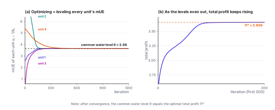
Optimization is the process of leveling every unit's mUE

The figure above records a full run of gradient ascent: four options start from wildly wrong prices, and their mUEs converge from every direction onto the same water level while total profit climbs steadily. After convergence I checked, and the common water level equals the optimal total profit (to within $10^{-14}$ ), exactly as the formula says.

Add a volume constraint and the structure stays the same. This matters — it shows how robust the knob is:

L = \sum_j q_ju_j + \lambda\Bigl(\sum_j q_j - Q\Bigr)

Using the last result of Section 3, $\sum_m \partial q_m/\partial p_j = -k_jq_jq_0$ :

\frac{\partial L}{\partial p_j} = q_j\bigl[1 - k_ju_j + k_j\Pi\bigr] - \lambda\,k_jq_jq_0 = 0

\Rightarrow\ \boxed{\ u_j - \frac{1}{k_j} \;=\; \Pi - \lambda\,q_0\ }

The right-hand side still doesn't depend on $j$ . The constraint doesn't change the "level every mUE" structure; it just lowers the water level a little.

5. How to read the result

$1/k_j$ is the markup an option naturally has room for.

It's measured in money. The smaller the price coefficient $k_j$ (the less users care about this option's price), the larger $1/k_j$ , and the more markup the option should carry. It's the ledger from the previous section seen from the other side: when users care little about price, winning one more sale means giving up a lot, so it pays to sell a bit less at a higher price.

Optimal price = common water level + the option's own natural markup + its own cost.

You can say this sentence to a business audience as is, and it's easy to accept: everyone shares one "baseline level of profitability", and each option shifts away from it according to how little its customers care about price and how much it costs.

It gives you a diagnostic you can use right away.

Take your current live prices, compute each option's $\mathrm{mUE}_j = (p_j - c_j) - 1/k_j$ , and sort:

mUE clearly above the rest → the option is overpriced: one more sale of it nets more than one more sale of anything else, so cut its price and sell more
mUE clearly below the rest → the option is underpriced: one more sale of it is worth less than elsewhere, so raise its price and let the volume go to others
The wider the spread, the farther you are from the optimum, and the more there is to gain

This check doesn't require re-solving the optimization problem. A single SQL query does it, which makes it a great fit for a daily monitoring dashboard.

It also explains why blanket discounts are a bad idea. A storewide 20% discount cuts each price by an amount proportional to its original price — expensive items drop a lot, cheap ones only a little — while $1/k_j$ stays put. The mUEs that were level get scattered, and you end up farther from the optimum. The right move is to shift the water level: add the same amount of money to every $p_j$ , or take the same amount off, instead of multiplying them all by the same discount.

A counterintuitive but useful result: in this model, moving every price by the same amount keeps the optimal structure intact (it only shifts the water level); applying the same percentage discount doesn't.

Price Optimization · Part 3 of 4

← Pricing Many Items Under Constraints　·　Series index　·　Pricing at Scale →

Revision history